Usage

Working with Impedances in Python

Building complex impedance models is surprisingly simple in Python when you get the hang of it! Here are the key principles:

Note: In our code implementation, we use JAX’s NumPy (jnp) instead of standard NumPy (np) because JAX provides automatic differentiation and just-in-time compilation. These make the computation faster.

Basic Rules

1. For components in series: Add the impedances (Z)

2. For components in parallel: Add the admittances (Y = 1/Z)

Example Usage

Let’s understand how to build circuit models, writing them in a natural way while following the format needed for the impedance agent:

# Example: RC parallel circuit in series with resistor
def rc_circuit(p, f):
    """
    RC circuit: Rs + (Rct || Cdl)
    Written naturally but formatted for impedance agent

    Parameters:
        p: [Rs, Rct, Cdl] - array of parameters
        f: frequencies
    """
    w = 2 * jnp.pi * f
    Rs, Rct, Cdl = p

    # Define circuit elements
    Zs = Rs                      # Series resistance
    Zrct = Rct                   # Charge transfer resistance
    Zcdl = 1 / (1j * w * Cdl)    # Double layer capacitance

    # Combine parallel elements (Rct || Cdl):
    Yrct = 1/Zrct               # Convert to admittance
    Ycdl = 1/Zcdl               # Convert to admittance
    Ytotal = Yrct + Ycdl        # Add admittances in parallel
    Zrct_cdl = 1/Ytotal         # Convert back to impedance

    # Add series resistance
    Ztotal = Zs + Zrct_cdl

    # Return real and imaginary parts concatenated
    return jnp.concatenate([Ztotal.real, Ztotal.imag])

Here’s another example with a Randles circuit including CPE and Warburg elements:

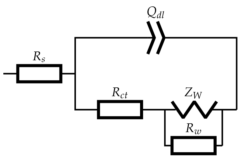
def randles_circuit(p, f):
    """
    Randles circuit with CPE and finite-length Warburg:
    Rs + (Qdl || (Rct + W || Rw))

    Parameters:
        p: [Rs, Q, n, Rct, W, Rw] - array of parameters
        f: frequencies

        Rs: Series resistance
        Q: CPE constant
        n: CPE exponent
        Rct: Charge transfer resistance
        W: Warburg coefficient
        Rw: Warburg resistance
    """
    w = 2 * jnp.pi * f
    Rs, Qdl, n, Rct, Wct, Rw = p

    # Define circuit elements
    Zs = Rs                                  # Series resistance
    Zcpe = 1 / (Qdl * (1j * w)**n)            # CPE impedance
    Zw = Wct / jnp.sqrt(w) * (1 - 1j)         # Warburg impedance

    # Combine Warburg with Rw in parallel
    Yw = 1/Zw                               # Warburg admittance
    Yrw = 1/Rw                              # Rw admittance
    Yw_total = Yw + Yrw                     # Parallel combination
    Zw_total = 1/Yw_total                   # Back to impedance

    # Add Rct in series with Warburg||Rw
    Zrct_w = Rct + Zw_total

    # Combine with CPE in parallel
    Yrct_w = 1/Zrct_w                       # Convert to admittance
    Ycpe = 1/Zcpe                           # CPE admittance
    Ytotal = Yrct_w + Ycpe                  # Parallel combination
    Ztotal = 1/Ytotal                       # Back to impedance

    # Add series resistance
    Z = Zs + Ztotal

    # Return real and imaginary parts concatenated
    return jnp.concatenate([Z.real, Z.imag])

Common Circuit Elements

# Resistor (R)
Z_R = R

# Capacitor (C)
Z_C = 1 / (1j * w * C)

# Inductor (L)
Z_L = 1j * w * L

# Warburg Element (W)
Z_W = W / np.sqrt(w) * (1 - 1j)

# Constant Phase Element (CPE)
Z_CPE = 1 / (Y0 * (1j * w)**alpha)

Command Line Interface

Basic Analysis

The CLI provides several options for analyzing impedance data:

# Basic analysis with default settings
impedance-agent analyze data.txt

# Analysis with custom ECM model
impedance-agent analyze data.txt --ecm model.yaml

# Analysis with specific LLM provider
impedance-agent analyze data.txt --provider deepseek

# Export results and generate plots
impedance-agent analyze data.txt --output-path results/analysis.json --plot

CLI Options

Arguments:
    data_path                Path to impedance data file

Options:
    --provider TEXT         LLM provider (deepseek/openai) [default: deepseek]
    --ecm TEXT             Path to the equivalent circuit model(ECM) configuration file
    --output-path TEXT     Path for output files
    --output-format TEXT   Output format (json/csv/excel) [default: json]
    --plot-format TEXT     Plot format (png/pdf/svg) [default: png]
    --plot                 Generate plots [default: True]
    --show-plots           Display plots in window [default: False]
    --log-level TEXT       Logging level
    --debug               Enable debug mode
    --workers INTEGER      Number of worker processes

Python API

Basic Usage

from impedance_agent import ImpedanceAnalysisAgent

# Initialize the agent with specific provider
agent = ImpedanceAnalysisAgent(provider="deepseek")

# Analyze data with built-in model
results = agent.analyze("data.txt", model="randles")

Complete Example

Here’s a complete example demonstrating impedance analysis with synthetic data:

import numpy as np
from impedance_agent.core.models import ImpedanceData
from impedance_agent.agent.analysis import ImpedanceAnalysisAgent

# Create sample data
freq = np.logspace(-2, 5, 50)
z_real = 1 + 2 / (1 + (2 * np.pi * freq * 1e-3) ** 2)
z_imag = -2 * 2 * np.pi * freq * 1e-3 / (1 + (2 * np.pi * freq * 1e-3) ** 2)
data = ImpedanceData(frequency=freq, real=z_real, imaginary=z_imag)

# Define ECM configuration
ecm_config = {
    "model_code": """
    def impedance_model(p, f):
        w = 2 * jnp.pi * f
        Rs, Rct, Cdl = p
        Z = Rs + Rct / (1 + 1j * w * Cdl * Rct)
        return jnp.concatenate([Z.real, Z.imag])
    """,
    "variables": [
        {"name": "Rs", "initialValue": 1.0, "lowerBound": 0, "upperBound": 10},
        {"name": "Rct", "initialValue": 2.0, "lowerBound": 0, "upperBound": 10},
        {"name": "Cdl", "initialValue": 1e-3, "lowerBound": 0, "upperBound": 1},
    ],
}

# Run analysis
agent = ImpedanceAnalysisAgent(provider="deepseek")
result = agent.analyze(data, ecm_config)

# Print results
print(result.summary)
if result.time_constant_analysis:
    print("\nTime Constant Analysis:")
    print(f"Matching score: {result.time_constant_analysis['matching_score']:.2f}")